ABBREVIATIONS

DH, double haploid; GEBV, genomic estimated breeding values; GPS, genomic and phenotypic selection; GS, genomic selection; He, expected heterozygosity; INRAE, Institut National de la Recherche en Agriculture, Alimentation et Environnement; OCS, optimal contribution selection; OHV, optimal haploid value; PS, phenotypic selection; QTL, quantitative trait locus; SNK, Student-Newman-Keuls; SNP, single nucleotide polymorphism; SSD, single seed descent; TBV, true breeding value; UC, usefulness criterion; UCPC, usefulness criterion parental contribution

INTRODUCTION

The objective of bread wheat breeding programs is to develop new varieties that outperform current varieties in terms of yield, adaptation, resistance to biotic and abiotic stresses, and/or end use qualities. A great challenge in plant breeding is to improve the genetic gain per unit of time for a given investment. To meet this goal, the optimization of resource allocation appears to be a key point. In addition, breeders must find a compromise between short-term genetic gain and the conservation of genetic diversity within their germplasm in order to guarantee long-term genetic gain [1].

Furthermore, the exponential decrease of genotyping costs, improvement of computing tools, data storage capacities and algorithms’ efficiency, and the development of new statistical methods have led to the development of a new powerful approach to optimize breeding schemes: genomic selection (GS). GS is a marker-based selection method that uses thousands to millions of molecular markers evenly spread along the genome to predict the genetic value of candidates to selection [2,3]. According to the breeder’s equation [4], GS could improve genetic gain by (i) accelerating genetic gain by shortening the breeding cycle, replacing field evaluation with genotyping at juvenile stage [5] for long-cycle plants like trees in particular, implement recurrent selection with rapid cycles in cereals with up to 3 steps of GS per year in greenhouse for maize for instance [6,7], (ii) decreasing the budget allocated to field evaluation by optimizing the number of genotypes and replicates per environment in the experimental design [8] and by this way increasing the size of the breeding program (number of crosses or progenies per cross), (iii) increasing genetic variance by optimizing mating to cumulate favourable alleles [9–12], (iv) increasing accuracy of selection. For wheat in particular, theoretical estimates of genetic gain showed that GS can accelerate recurrent selection using off-season field for spring wheat or rapid cycles in greenhouses for winter wheat. The gain was higher when applying GS in F2 compared to F3 or F4 [13]. We can postulate that optimized mating should increase the gain further.

Several factors influence the accuracy of GS. These factors include trait architecture and trait heritability [14], training set size and composition [15,16], i.e., congruency between the allelic composition represented in the training population to estimate marker effects and the allelic composition of the candidates whose performance is to be predicted [17–23], marker density [23–26], and statistical model for estimation of marker effects [27]. For wheat in particular, it was shown that the size of the training population should be 50 if individuals are full-sibs, 100 if they are half-sibs and 1000 if they are unrelated [13].

Most of previous researches on GS in plant breeding focused on the prediction accuracy of unphenotyped lines. In bread wheat, studies evaluated the prediction accuracy of grain yield [28–32], traits linked to bread making quality [33–38], or disease [39–42]. At the breeding program scale, some simulation works showed an interest of GS compared to classical phenotypic evaluation in terms of genetic gain. For example, a study [43] showed that GS accuracies were high enough (GS accuracy twice as high as PS accuracy) to achieve greater gain from selection per unit time compared with phenotypic selection for bread wheat adult stem rust resistance. However, the two strategies they compared represented different budgets. In contrast, another study [44] simulated and compared several hybrid and line wheat breeding programs using GS for a fixed budget. This study showed that GS could be advantageous in terms of genetic gain for line but even more for hybrid breeding in wheat. Furthermore, the efficiency of PS and GS for grain yield assuming a single selection cycle and a given budget were compared using a biparental population of maize double haploid (DH) lines, as discussed by [45]. They showed that with large Genotype × Environment interactions and under limited resources, it was beneficial to use an index combining PS and GS to maximize genetic gain. They also noticed that DH price was a limiting factor for large genetic gain. But none of those studies evaluated the interest of mating optimization using genomic predictions. In maize, several studies showed its interest for long term genetic gain, in pre-breeding programs in particular [46–50].

Simulation studies actually enable the comparison of a wide range of scenarios that would not be possible to test experimentally. They also allow to evaluate an unlimited number of selection cycles (long-term selection) in a short amount of time with a cost limited to data storage and processing.

In this study we compared the genetic gain and the evolution of genetic diversity in two types of simulated breeding schemes: one called Phenotypic Selection (PS) with two steps of selection based on field trials, and one called Genomic and Phenotypic Selection (GPS) that combines a first step of genomic selection and a second step of selection based on field trials. We also evaluated the interest of mating optimization (GPSopt). We explored different scenarios in order to investigate under which conditions GPS and GPSopt were more cost-effective than PS. We compared scenarios for a given budget covering all breeding costs.

MATERIALS AND METHODS

We developed a R pipeline to simulate and compare winter wheat breeding programs in terms of genetic gain and genetic diversity evolution for a given budget (Figure 1). The scripts of the pipeline are available using the following link: https://forgemia.inra.fr/umr-gdec/gps.

FIGURE 1

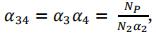
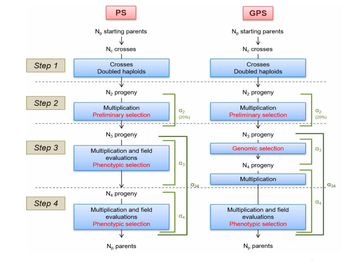Figure 1. PS and GPS breeding schemes. PS: Phenotypic Selection. GPS: Genomic and Phenotypic Selection. N_p and N_c: number of parents and crosses respectively. N₂, N₃ and N₄: number of progenies at the beginning of steps 2, 3 and 4 respectively. α₂, α₃ and α₄: selection rate on steps 2, 3 and 4 respectively. α₃₄: global selection rate on steps 3 and 4.

The pipeline was tested using a real breeding population of 757 winter-type bread wheat lines developed by the Institut National de la Recherche en Agriculture, Alimentation et Environnement (INRAE, formerly INRA) and its subsidiary company Agri-Obtentions. These lines were selected between 2000 and 2013. Each line was genotyped using a 280K SNP array [51]. The datasets with the genotyping data are available in the INRAE Dataverse repository (https://data.inrae.fr/dataset.xhtml?persistentId=doi:10.15454/M8SAYH). In order to limit computing time in simulation, we used a subset composed of 12,119 SNP evenly spread along the genetic map. Such marker number was previously shown as giving similar predictive ability as the full marker set [52].

We considered that 100 QTLs control the traits of interest. We simulated 20 traits using random positions of the 100 QTLs, i.e., 20 random samples of 100 SNPs were assigned as QTL, marker effects drawn from a gaussian distribution:

β~N(0,1)

The favourable allele was attributed at random to one of the two SNP alleles, so that coupling and repulsion associations also occur at random. The entry-mean heritability (h²) was set to either 0.2, 0.4 or 0.7. Phenotypic values of lines were obtained by adding a normally distributed noise to the genotypic values. In our study, the residual variance was 80% (h² = 0.2), 60% (h² = 0.4) or 30% (h² = 0.7) of phenotypic variance. We simulated phenotypes as:

(1)

with Q the genotyping matrix of 100 QTLs and β the vector of marker effects.

We compared two types of breeding schemes (Figure 1): one called Phenotypic Selection (PS) with two steps of selection based on field trials, and one called Genomic and Phenotypic Selection (GPS) that combines a first step of genomic selection and a second step of selection based on field trials. For the sake of simplicity, both breeding programs were designed using doubled haploids (DHs), instead of successive selfing, to reduce the time required for inbred development. We counted three years for cross, DH productions from F1 and seed multiplication, one year of PS (or GPS) selection and a last year of phenotypic selection, to fit breeder’s requirement of having real data to apply candidates in official registration trials. For both PS and GPS approaches, a breeding cycle lasts five years. We simulated three successive cycles. For the first cycle, the training population is composed of 757 N_ref lines that have been genotyped and virtually “phenotyped” for one trait (20 times). Then, we extend the training population at each cycle with the N₄ individuals that are genotyped and “virtually” phenotyped to update the genomic prediction equation.

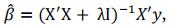
We start the simulation with N_ref lines (757 in our example) that have been genotyped and virtually “phenotyped” for one quantitative trait, twenty times to avoid any bias in QTL positions. For GPS, the first vector of marker effects is calculated using a ridge regression on those phenotypes. The database of phenotypes is incremented at each phenotyping step and the vector of marker effects is updated at each cycle k.

(2)

with y the vector of phenotypes, X the matrix of the 12,019 markers after removing the 100 markers sampled to simulate QTLs, λ chosen to make X’X non-singular, using the R package rrBLUP.

We evaluated the accuracy of genomic predictions using the correlation between TBV and GEBV of lines at the third step.

At the first step of each cycle, N_C crosses are produced between the N_P best individuals according to phenotyping results at step 4 of previous cycle (or N_ref individuals for the first cycle). In PS scheme, crosses are obtained by randomly mating these N_P best individuals. Note that we could have chosen to cross the two best individuals according to phenotypes, or the first with the second, the second with the third. But none of those strategy is realistic. In a real breeding program, breeders would select parents that complement for different traits. More realistic mating scenarios in PS strategy will be tested when a multi-trait strategy will be implemented in the pipeline. For this paper, we decided to compare PS and GPS strategy using the same random mating strategy among the N_P best individuals, and a GPS strategy with random or optimized mating. This second strategy is called GPSopt and optimizes the complementarity between parental alleles [53]. We calculate the value of a cross as the value of the individual that would have inherited the best chromosomes of its parents.

(3)

with UC_ij the usefulness criterion of the cross between the i-th and the j-th parents, i ≠ j, c the chromosome number, GEBV=. This UC assumes chromosome being inherited without recombination, which is true for half of the chromatids in a single meiosis, as it is the case for doubled haploids from F1. The best cross is the cross that could produce the best possible gamete if the progeny size was unlimited. This is unrealistic but it was shown to be an acceptable approximation of cross value when using DH in wheat programs by [53].

To simulate progeny, each chromosome is either parental or recombined. If recombined, the number of cross-overs on each chromosome is sampled from a Poisson distribution, and cross-overs positions are distributed randomly along the genetic map [51].

At step 2, N₂ progeny are multiplied to implement one trial at the following step. We considered that the selection at this step was made on agronomic visual traits, excluding plants with major defaults, disease sensibility in particular. Since it cannot be focused on targeted traits (yield), we considered it had no impact on the distribution of genetic value of the N₃ selected progeny. So, the selection was considered random for the targeted trait.

At step 3, N₃ progeny are evaluated in one trial.

N₃ = N²α₂(4)

with α₂ the selection rate at step 2 (α₂ = 0.2 in this study).

In PS scheme, these individuals are evaluated in the field and we consider a multiplication cost corresponding to five trials for next step. Selection is based on phenotypic data with a rate of selection α₃. In GPS scheme, there is no trial, the selection is based on GEBVs calculated as the cross product between the vector of marker effects and the matrix of genotypes of progenies, excluding markers to which QTLs were assigned. Only N₄ (N₃α₃) progeny are multiplied in nursery.

At step 4, N₄ progeny are evaluated in five trials (different environments, e.g., different locations).

N₄ = N³α₃(5)

The last step is a phenotypic selection of N_P parents for the next cycle in both PS and GPS schemes with a selection rate α₄.

N_p = N⁴α₄(6)

Instead of defining α₃ and α₄ independently, we fixed a relative selection rate (called λ) between steps 4 and 3 as follow:

α₃=α₃₄^λ(7)

and

α₄=α₃₄^1-λ(8)

with:

(9)

If λ = 0.5, α₃= α₄. If λ > 0.5, α₃< α₄. If λ < 0.5, α₃ > α₄.

We defined C_x the cost of each operation X of the breeding program (Supplementary Table S1). The cost of an operation sometimes varies depending on the step where the operation was done. The step is then specified as an exponent. For example, we assumed that field evaluations were realized in one trial at step 2, five trials at step 3 and ten trials at step 4 (for registration), which explains the different costs of seed multiplication and evaluation. Note that those costs that include DNA extraction, genotyping and biometrician salaries are specific to INRAE. Genotyping cost may decrease in the future. Some other genotyping platforms are more flexible and allow to genotype with high density the parents and low density the progeny that can be imputed [13].

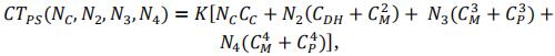
Total cost (CT) of the PS scheme was defined as follow:

(10)

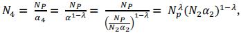
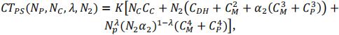
with K the number of cycle (K = 3 in this study) and N₂ the progeny number at the beginning of step 2. In our study, we supposed that the number of progenies was the same for all crosses. Note however that the pipeline offers the possibility to make it proportional to cross value (Usefulness Criterion). Total cost depends on 4 parameters concerning progeny size at each step. The number of possible combinations for a same budget is very large. In order to simplify comparisons, as progeny sizes are dependant of each other for a fixed budget, we defined three parameters (N_C, N_P and λ) that are fixed for one scenario. The total cost CT and progeny sizes N₃ and N₄ can be expressed as functions of these parameters and N₂.

Thanks to previous equations, we have:

(11)

Therefore, the total cost of the PS scheme can be defined as follows:

(12)

For a given total cost and set of parameters (N_C, N_P and λ) we search for the value of N₂ that solve this equation.

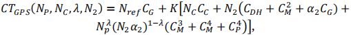
To define the total cost of the GPS scheme (CT_GPS), we introduced the genotyping cost of the reference population composed of N_ref lines. Note that cost of field evaluation at the third step is replaced by the cost of genotyping and that only N₄ lines that are selected at step 3 were multiplied for GPS (instead of N₃ for PS):

(13)

As genotyping cost is lower than phenotyping cost, the number of progenies is larger in GPS strategy. As we fixed the total cost, either the number of crosses or the number of progenies per cross will be different between PS and GPS schemes. For GPS and GPSopt schemes, we tested scenarios with the same number of crosses and a different number of progenies n2 per cross (called GPS.n2 and GPSopt.n2) and scenarios with the same number of progenies per cross and a different number of crosses (called GPS.N_C and GPSopt.N_C).

We evaluated the impact of several parameters on the final genetic gain. To do so, we simulated breeding programs with two total costs for 15 years (three cycles of five years; CT ∈ {22.5 M€, 45 M€}, i.e., average CT per year of 1.5 or 3 M€), two genotyping cost (CG ∈ {37€, 10€}), three relative selection rate λ (λ ∈ {0.25,0.5,0.75}), and three levels of heritability of the trait (h² ∈ {0.2,0.4,0.7}). The description of each scenario is available in Supplementary Table S2.

It led to the evaluation of 36 scenarios for five different strategies (PS, GPS.n2: fixed number of crosses, GPS.N_C: fixed number of progenies per cross, GPSopt.n2: optimized mating design with a fixed number of crosses, GPSopt.N_C: optimized mating design with a fixed number of progenies per cross). For each strategy / scenario, we tested 20 simulated traits (100 QTLs randomly sampled for each simulated trait) to evaluate the variance due to different QTL positions. For each combination of strategy, scenario and trait, we ran the algorithm 10 times to estimate the variance due to mendelian sampling only. For each simulation, we performed three cycles of five years.

The algorithm used to run the simulations required several input data: including the simulated strategy (PS, GPS.N_C, GPS.n2, GPSopt.N_C, GPSopt.n2) trait and replication, a matrix with chromosome number and genetic position in columns 1 and 2 respectively, a matrix of genotypes with N_ref rows, a vector of phenotypes of N_ref length, one vector including true marker effects for the simulated trait, one scenario (combination of CT, C_G, λ and h² values), the cost of each operation and the selection rate on step 2. The algorithm is illustrated in Supplementary Figure S1.

For each strategy and scenario, at the end of each cycle, we computed the genetic gain as the difference between the mean of the true breeding values (TBVs) of the N_p (200) best lines and the reference (initial) data set. The average TBV of the 200 best parental lines was 4.85. This average TBV was higher than the average TBV of the parental population which was 0.33. We performed an analysis of variance (ANOVA) to compare the impact of the input parameters on the genetic gain.

We tested a model without interactions between parameters (14), models that take into account interactions between the strategy and the simulated trait (15), the strategy and the total cost of the breeding scheme (16), the strategy and the relative selection rate (λ) (17), the strategy and the trait heritability (18).

g_ijklm = µ₀ + S_i + λ_j + h²_k + CT_l + T_m + ε_ijklm,(14)

g_ijklm = µ₀ + S_i + λ_j + h²_k + CT_l + T_m + S_i x T_m + ε_ijklm,(15)

g_ijklm = µ₀ + S_i + λ_j + h²_k + CT_l + T_m + S_i x CT_l + ε_ijklm(16)

g_ijklm = µ₀ + S_i + λ_j + h²_k + CT_l + T_m + S_i x λ_j + ε_ijklm(17)

g_ijklm = µ₀ + S_i + λ_j + h²_k + CT_l + T_m + S_i x h²_k + ε_ijklm(18)

with g_ijklmn is the genetic gain of the scenario with the the i-th strategy (S), the j-th value of λ, the k-th value of h², the l-th value of CT, and for the m-th simulated trait (T).

For GPS strategies, we also studied the impact of genotyping cost on genetic gain:

g_ijklm = µ₀ + S_i + λ_j + h²_k + CT_l + T_m + S_i x CG_n + ε_ijklm(19)

with CG_n the n-th value of CG. F tests were considered significant at α < 0.05.

For the different strategies, genetic gains for pairwise scenarios were compared using the Student-Newman-Keuls (SNK) test from the R library Agricolae. Means were judged significantly different when P-values < 0.05.

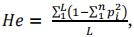
For each strategy and scenario, we analysed the evolution of genetic diversity over successive cycles. To do so, we measured the percentage of alleles present in both the reference population and the 200 best progenies of each cycle. We estimated the significance of the various factors on genetic diversity with the same models used for genetic gain above. We also measured the difference between the expected heterozygosity (He) in the initial population and at the third cycle for (i) all the markers but QTLs, (ii) markers assigned to QTLs and (iii) markers located at the vicinity of QTLs (positioned at less than 1, 5, 10 or 15 cM from a QTL), using the following formula:

(20)

with L the number of loci, n the number of alleles (2 in our case) for each locus, and p_i the frequency of the allele i.

For the different strategies, He differences at the end of the last cycle were compared using the SNK test.

We also compared the number of cumulated favourable alleles (difference between the third cycle and the initial population) between strategies and scenarios.

For GPSopt strategies, a usefulness criterion was used to choose crosses that maximize the probability to get lines that cumulate a maximum of favourable alleles among the N_p selected lines. Note that in our example, we did not constrain the contribution of any parents, but it is possible to fix a contribution threshold using this pipeline. For GPS and PS strategies, crosses were chosen at random among the N_p selected lines.

We compared the distribution of the contributions of reference lines between strategies and scenarios based on the pedigree of the N_p lines selected at the end of each cycle.

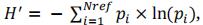
We defined the contribution of a reference line as the number of selected progenies presenting them in their pedigree divided by the total number of parental lines that contributed to the global progeny. Note that all the reference lines or N_p lines selected at the end of previous cycle did not contribute to crosses. Then we calculated the number of parents that contributed to 25% and 75% of the progeny. In addition, we used the Shannon index to evaluate the diversity of the parental lines that contributed using the following formula:

(21)

with N_ref the number of initial parental lines, and p_i = n_i/N with n_i the contribution of parent i to the N_p progenies and N the total number of lines that contributed to progeny. Note that the more unequal the parental contributions, the smaller the corresponding Shannon index.

In order to check if the distribution of favourable alleles was different among parents selected by UC or at random, we computed for each cross that contributed to selected lines the number of shared and specific favourable alleles among the two parents. We calculated it for each cycle.

RESULTS

When the budget CT was doubled, the number of progenies was 1.9 times larger at each step on average (for given values of C_G and λ). When the cost to genotype one line (C_G) decreased from 37 to 10 euros, the number of progenies at each step was only 1.1 times larger at each step on average (for given values of CT and λ). Note that for given values of CT and C_G, the higher the value of λ, the higher the population size N₃ in step 3, the smaller the population size in step 4 N₄ and the higher N₃ + N₄.

Supplementary Table S3 reports the number of progenies at each step, for each strategy (PS, GPS.N_C, GPS.n2, GPSopt.N_C, GPSopt.n2) and scenario (combination of CT, C_G and λ).

We compiled the percentage of the total budget allocated to each operation (crosses, DH, multiplication, field experiment and genotyping) under different strategies (PS, GPS.N_C, GPS.n2, GPSopt.N_C, GPSopt.n2) and scenarios (combination of CT, C_G, λ). Results were similar for GPS.N_C and GPS.n2, and for GPSopt.N_C and GPSopt.n2, for that reason we only show results for PS, GPS.n2 and GPSopt.n2 in Table 1. For each strategy, the production of DHs was the major source of expenses. Indeed, for PS strategy between 30.8% and 46.5% of the global budget was allocated to DH production. This percentage is even higher for GPS schemes (between 37.3% and 72.6%). Multiplication steps required on average between 20% and 25% of the global budget. Since one field evaluation was more expensive at step 4 than at step 3 (more replicated plots), scenarios with a higher number of lines in the last step (λ < 0.5) used more budget for field evaluations.

For GPS strategies, genotyping required between 7.6% and 13.1% of the global budget when the cost of genotyping was 37€. It was obviously lower when the cost of genotyping was 10 € (ranging from 2.2% to 3.9%). But note that the number of tested lines only slightly increased (x1.1).

TABLE 1

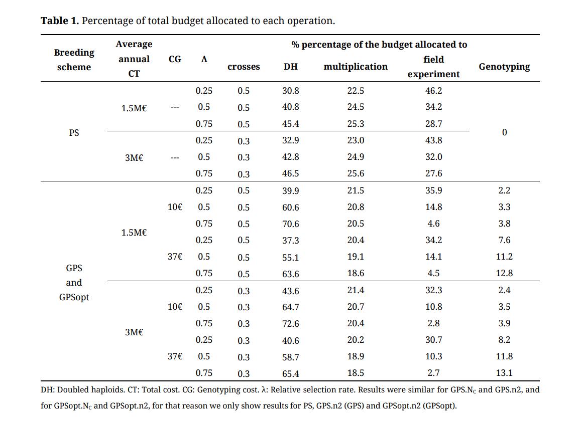Table 1. Percentage of total budget allocated to each operation.

We evaluated the contribution of input parameters (i.e., strategy, total cost, trait heritability, QTL sampling, and λ) to genetic gain for the 200 lines selected at last step.

We found that each of the five factors had a significant effect on the final genetic gain (Supplementary Table S4). Trait heritability contributed the most. As expected, scenarios with higher heritabilities led to higher genetic gain (the average genetic gain was 13.32, 16.36 or 18.90 when the heritability was 0.2,0.4 or 0.7, respectively). The strategy was the second most significant parameter. The genetic gain for GPSopt.N_C and GPSopt.n2 strategies was larger than the genetic gain for strategies using random mating (the average genetic gain was 18.0 for GPSopt, 15.0 for GPS and 15.3 for PS). The strategy and the trait heritability accounted for 16.7% and 40.1% of the sum of squares, respectively. Note that doubling the total cost had a rather low impact on the final genetic gain (+ 1.07 on average). In addition, λ and QTL sampling had a low impact on the final genetic gain. We did the same analysis with the genetic gain obtained for various selection rates at last step (for the 10, 50 and 100 best lines) and we obtained the same conclusions (Supplementary Table S5). For GPS strategies, decreasing genotyping cost from 37€ to 10€ had no significant effect on the genetic gain (the average genetic gain was 16.4 for 37€, 16.5 for 10€).

TABLE 2

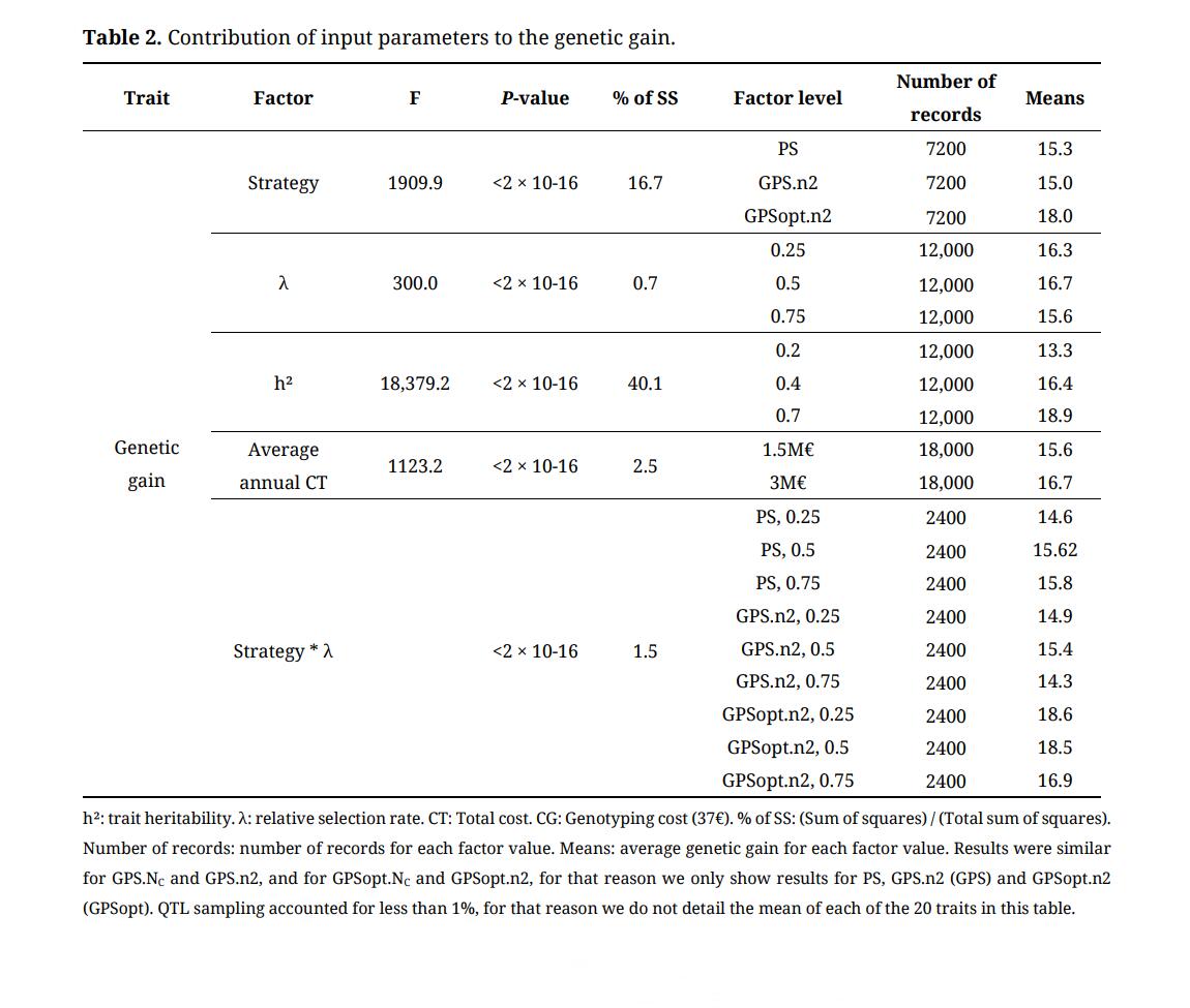Table 2. Contribution of input parameters to the genetic gain.

Considering the interaction between strategy and one of the other input parameters, we found that strategy and λ had the most significant effect on final genetic gain (Table 2). The genetic gain for GPS strategies (GPS.N_C, GPS.n2, GPSopt.N_C and GPSopt.n2) was always larger than genetic gain for PS when λ = 0.25 (i.e., α₃> α₄, N₃ is decreased and N₄ is increased compared to λ = 0.75, the selection is less stringent at step 3 where GPS is applied). The interaction between strategy and total cost and the interaction between strategy and trait heritability had a significant effect on final genetic gain but they accounted for less than 1% of the sum of squares. Finally, the interaction between strategy and QTL sampling (i.e., the simulated trait) had no significant effect on final genetic gain.

As expected, we observed an increase of the 200 best lines average TBV along generations. Figure 2 illustrates the cumulative genetic gain at the end of each cycle with an average annual CT = 3M€ and C_G = 37€. Results for other values of CT and C_G are available in Supplementary Table S6.

Genetic gain was always significantly larger for GPSopt.N_C and GPSopt.n2 than for PS, GPS.N_C and GPS.n2 whatever the values of CT, λ, CG and h². The difference between GPSopt.N_C or GPSopt.n2 and PS was even larger when λ = 0.25 ( α₃ > α₄). Indeed, the average differences between GPSopt and PS were + 3.94 for λ = 0.25, +2.90 for λ = 0.5 and +1.46 for λ = 0.75 (Table 2). Genetic gain was also larger for GPS.N_C and GPS.n2, compared to PS when λ = 0.25. However, this difference was significant in only one third of the scenarios. When λ = 0.5, no significant difference was observed between PS, GPS.N_C and GPS.n2. In contrast, when λ = 0.75, genetic gain was significantly larger for PS compared to GPS. N_C and GPS. n2 (+ 1.55).

Note that GPS. N_C and GPSopt. N_C allowed to do 156 more crosses per cycle on average compared to GPS. n2 and GPSopt. n2. The number of progenies per cross was decreased from 412 to 333 for n3 and from 82 to 67 for n4 (with λ = 0.25, average annual CT = 3 M€ and CG = 37€). However, the genetic gain for GPS. N_C (GPSopt. N_C) and GPS.n2 (GPSopt. n2) was not significantly different whatever the scenario.

FIGURE 2

Figure 2. Evolution of genetic gain. h²: trait heritability. λ: relative selection rate. Average annual total cost (CT) = 3M€ and genotyping cost (CG) = 37€. Results were similar for GPS.N_C and GPS.n2, and for GPSopt.NC and GPSopt.n2, for that reason we only show results for PS, GPS.n2 (GPS) and GPSopt.n2 (GPSopt).

We calculated the Pearson correlation between TBV and GEBV (GS accuracy) and between TBV and phenotypic values (PS accuracy) for the progenies at step 3 (Table 3). As expected, accuracy increased with trait heritability. Whatever the values of trait heritability and λ, PS accuracy at step 3 slightly decreased over the cycles. In contrast, GS accuracy increased over cycles. For instance, for GPSopt strategies, accuracy at step 3 of third cycle was on average twice as high as the one at the first cycle. Although λ had low impact on PS accuracy, it was significant on GPS and GPSopt. When λ = 0.25 (α₃> α₄), final accuracy was superior compared to scenarios with λ = 0.75 (+ 0.12 and + 0.17 in GPS and GPSopt respectively). When λ decreases, the number of progenies N₄ evaluated in the field at step 4 increases (Supplementary Table S3) and the number of lines added to the training population increases.

TABLE 3

Table 3. PS and GS accuracies at step 3.

As expected, we observed a decrease of polymorphism rate (calculated as the percentage of alleles present in both the reference lines and the selected progenies) over cycles for all scenarios and strategies.

The five input factors had a significant effect on polymorphism rate (percentage of alleles) in the 200 best progenies of the last cycle compared to the reference (initial) population (Supplementary Table S8). Figure 3 illustrates the results with an average annual CT = 3M€ and CG = 37€. Results for other values of CT and CG are available in Supplementary file. Each of the five factors had a significant effect. Strategy and λ accounted for 39.1% and 13.7% of the sum of squares, respectively. Trait heritability, annual total cost and QTL sampling (the simulated trait) accounted for less than 1% of the sum of squares. This decrease was more pronounced for GPS breeding schemes than for PS, when crosses were optimized in particular, and when λ = 0.75.

FIGURE 3

Figure 3. Evolution of polymorphism rate over cycles. h²: trait heritability. λ: relative selection rate. Annual total cost (CT) = 3 M€ and genotyping cost (CG) = 37€. The evolution of polymorphism rate was calculated as the percentage of alleles present in both the reference population and the selected progenies. Results were similar for GPS.N_C and GPS.n2, and for GPSopt. N_C and GPSopt. n2, for that reason we only show results for PS, GPS. n2 (GPS) and GPSopt. n2 (GPSopt).

We also estimated the evolution of the expected heterozygoty (He) over the cycles (Supplementary Table S7) and the difference He in the reference population and at the end of each cycle for the all set of markers except QTLs, for markers assigned to QTLs and for markers at the vicinity of QTLs (1, 5 and 10 cM) (Table 4). Initial He in the reference population (He_ini) was 0.26. He decreased faster for GPSopt strategies (−0.14 < effect at the end of third cycle < −0.09) whatever the scenario compared to GPS strategies (−0.08 < effect < −0.03) and PS strategy (−0.03 < effect < −0.02). The difference was even larger when λ = 0.75 for GPS strategies (−0.14 < effect < −0.12 for GPSopt, −0.1 < effect < −0.08 for GPS). The loss of genetic diversity was stronger at QTL locations but not at the vicinity of QTLs.

The number of additional favourable alleles cumulated at the end of the third cycle was also significantly larger for GPSopt strategies. For GPSopt, it ranged from 15.57 for h² = 0.2 and λ = 0.75 to 22.39 for h² = 0.7 and λ = 0.25. For GPS, it ranged from 13.2 for h² = 0.2 and λ = 0.75 to 19.1 for h² = 0.7 and λ = 0.5. For PS, it ranged from 12.75 for h² = 0.2 and λ = 0.25 to 19.47 for h² = 0.7 and λ = 0.75.

TABLE 4

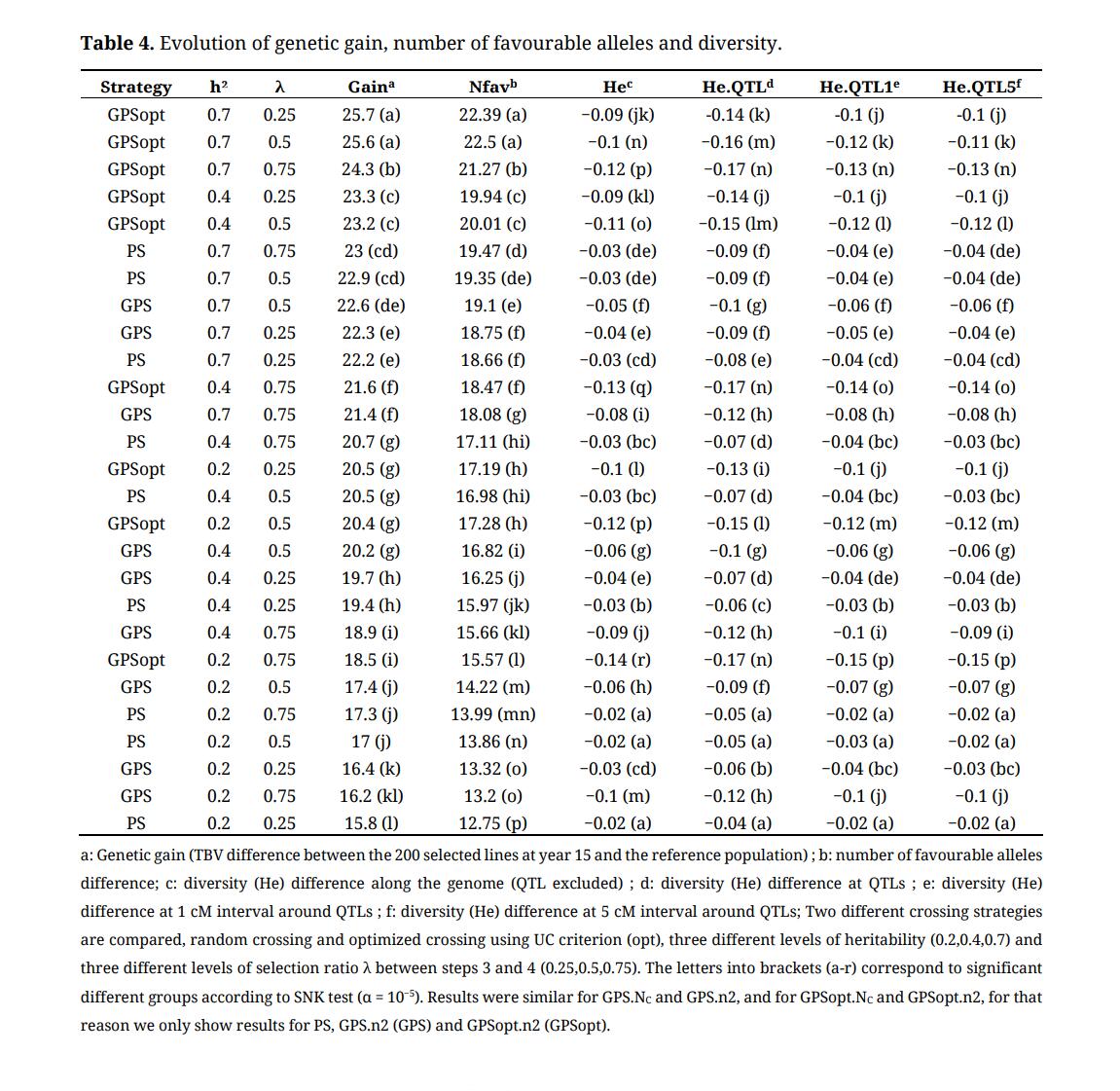Table 4. Evolution of genetic gain, number of favourable alleles and diversity.

The number of reference lines that contributed to progenies decreased over cycles (Supplementary Table S9). When average annual CT = 3 M€ and C_G = 37€, on average 31 reference (founder) lines were used as parents to produce the 200 best lines of the last cycle in GPSopt strategies. In contrast, on average 53 founder lines were used as parents in other GPS strategies and 81 in PS strategy. We also noticed that the number of founder lines was slightly smaller for GPS strategies with 400 crosses (GPS.N_C and GPSopt.N_C) compared to GPS strategies with more crosses (GPS.n2 and GPSopt.n2).

We also calculated the number of reference lines that contributed to 25% or 75% of progeny. These two indicators followed the same trends as the number of reference lines that contributed to the whole progeny (Supplementary Table S9). Indeed, only 1.4 reference lines contributed to 25% of progeny for GPSopt strategy on average compared to 3.2 and 4.8 different initial lines were needed in GPS and PS strategies, respectively. On average, 7 founders contributed to 75% of progeny, compared to 17 and 27.6 for GPS and PS strategies, respectively. These reveals that some parents contribute to a large number of selected progenies for GPSopt if no contribution threshold is applied. This is consistent with the Shannon index that was smaller for GPSopt approach at the end of the third cycle (2.4,3.3 or 3.8 in GPSopt, GPS or PS).

TABLE 5

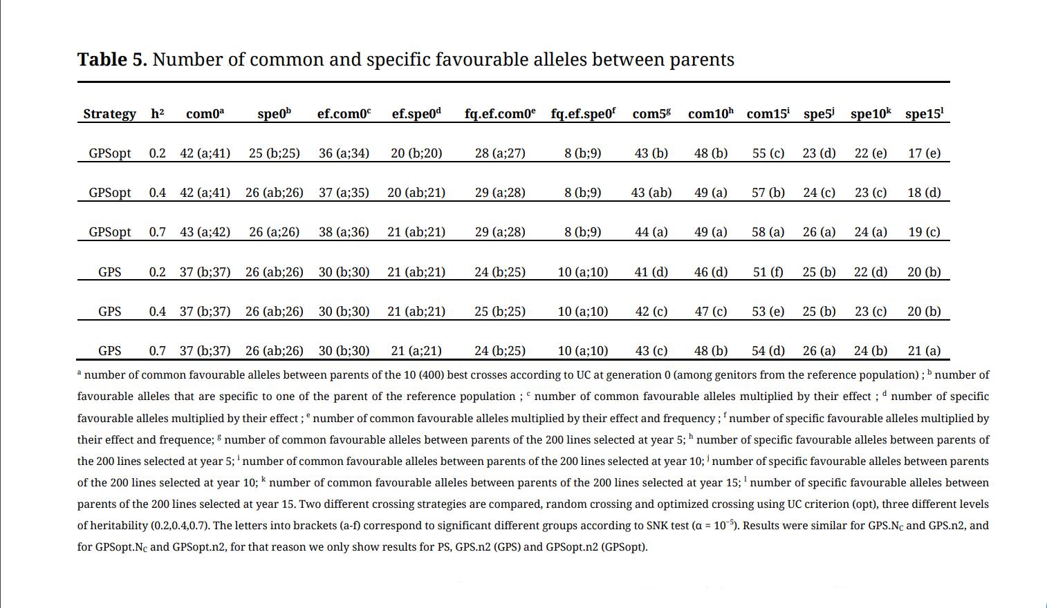Table 5. Number of common and specific favourable alleles between parents.

We also observed that the number of favourable alleles present in both parents was larger in GPSopt compared to the other strategies (Table 5) and that this number increased over cycles. On the opposite, the number of favourable alleles specific to one parent was not different between optimized and random crossing strategies in our elite germplasm (reference population) but became significantly inferior over cycles as the number of favourable alleles and inbreeding increased. There was 5 more QTLs in common between parents at the first generation in GPSopt compared to GPS, 4 more at the third cycle (year 15). Finally, GPSopt was more efficient to increase the frequency of favourable alleles, especially when those alleles were rare in the reference population, heritability was high and λ was low (α₃ was high) (Figure 4).

FIGURE 4

Figure 4. Increase of favourable alleles frequency. h²: trait heritability. λ: relative selection rate. Annual total cost (CT) = 3 M€ and genotyping cost (CG) = 37€. Results were similar for GPS.N_C and GPS.n2, and for GPSopt.N_C and GPSopt.n2, for that reason we only show results for PS, GPS.n2 (GPS) and GPSopt.n2 (GPSopt).

DISCUSSION

This study focused on two types of breeding schemes: Phenotypic Selection (PS) with two steps of selection based on field trials, and Genomic and Phenotypic Selection (GPS) that combines a first step of genomic selection and a second step of selection based on field trials. We finalized the cycle by phenotypic selection because plant breeders have to provide field data for candidates when applying for official variety registration. In order to compare PS and GPS schemes with a fixed budget, GPS could either have the same number of crosses than PS (GPS.n2) or it could have the same number of progenies per cross at the beginning of step 2 (GPS.N_c). In addition, we explored two methods to choose couples to be crossed at each cycle for GPS schemes: random mating of the best lines (GPS.N_C or GPS.n2 strategies) or optimized mating (GPSopt.N_C or GPSopt.n2 strategies) using the optimal haploid value (OHV) usefulness criterion [53]. We tested several scenarios by varying cost of the breeding scheme, genotyping cost, trait heritability and selection rates at each step of selection, in order to investigate under which conditions GPS was more efficient than PS. We evaluated each strategy by comparing the genetic gain of lines selected at the end of the breeding program and the evolution of genetic diversity over cycles. Note that computational time was three to five times longer for the simulations of breeding schemes with optimized mating.

The objective of bread wheat breeding programs is to develop new varieties that outperform existing varieties, particularly those used as control in official registration trials. To reach this goal, breeders have to choose the strategy that leads to maximal True Breeding Value (TBV, with the hope that the realized phenotype will also be superior. As expected, the TBV of the 200 best lines increased over cycles for all strategies and scenarios in our simulations.

We observed that trait heritability and strategy (PS, GPS, GPSopt) are the two main factors affecting genetic gain which is consistent with the breeder’s equation [4]. To a lesser extent, relative selection rate (λ) between genomic and phenotypic selection steps had a significant effect on the genetic gain variance.

In this study, we simulated traits controlled by 100 QTLs randomly sampled from 12,119 genomic markers. The next step will be to vary the number of sampled QTLs, the distribution of their effects and epistasis.

We simulated breeding programs with two different budgets. Doubling the global budget did not lead to a large increase of the genetic gain (+ 6% on average). The genotyping cost had no significant effect on the genetic gain variance. This may be due to DH expense that is so high that varying the other costs has low impact on progenies number. This suggests that the INRAE-AO breeding program and reference panel may not have reached the necessary critical size to benefit fully from genomic predictions.

We however identified under which conditions genomic predictions were the most interesting. We compared two strategies, genotyping predictions were used (1) to select candidates for next steps (GPS.N_C and GPS.n2 strategies), or (2) to select candidates and optimize crosses (GPSopt.N_C and GPSopt.n2 strategies). In our germplasm, we found that only strategies with optimized crosses were significantly superior to PS in terms of final genetic gain. We showed that parents involved in crosses that have led to the production of selected lines had a larger number of favourable alleles when the crosses were optimized. In addition, we highlighted the fact that some parents were involved in a large proportion of crosses in GPSopt strategies, leading to efficient favourable allele frequency increase, even rare alleles, but also global decrease of diversity and a genetic gain slowdown. Strategies with optimized mating were more advantageous when the selection rate was more intense at the step of phenotypic selection (step 4) than at the step of genomic selection (step 3). In this case, the number of progenies that were both genotyped and phenotyped at each cycle in GPS and GPSopt strategies were larger. As genomic prediction equations were updated at each cycle, the training population was larger and the predictions were more accurate. This result is consistent with previous studies that have shown that training population size and composition are key factors affecting accuracy of genomic predictions [15,16].

In our simulations GPS and PS breeding programs required the same number of years. It would be interesting to simulate more realistic breeding programs were genomic predictions results in accelerating the breeding programs using rapid cycles for instance [44,54,55].

Genetic diversity is a key parameter in plant breeding since it has an effect on long term genetic gain (according to breeder’s equation [4]). However, it has been shown in both experimental study and by stochastic simulations [1,56] that GS accelerates the loss of diversity compared to phenotypic selection due to the rapid fixation of regions of the genome with an effect on the trait of interest. Our results were consistent with those studies. Indeed, we observed a faster decrease of polymorphism rate in GPS strategies compared to PS schemes whatever the simulated scenario. This loss of alleles was even faster for strategies with optimized crosses (GPSopt.N_C and GPSopt.n2). In order to reduce this loss, we could place additional weight on low-frequency favourable alleles as recommended by [1]. Since the loss of diversity is particularly fast when crosses were optimized, a second option would be to define a maximum number of crosses for which each parent could contribute in order to avoid having too many lines with one (or two) common parent like the optimal contribution selection (OCS) strategies [49]. Note that favourable alleles were more efficiently fixed for GPS and GPSopt and the frequency of favourable alleles, the rare ones in particular increased faster. In this study, we considered that only lines from the previous generation could be mated. This assumes no introduction of neo-diversity in the breeding scheme, which is not realistic, but simulations are always a simplification of real life. Indeed, it is common use to introduce external bread wheat registered material at each cycle. In order to simulate more realistic breeding programs, it would be important to give the possibility to add parents from an external pool (for example lines selected by other breeders or coming from genetic resources collections).

A great challenge in plant breeding is to improve and accelerate the genetic gain with a fixed budget. To meet this goal, breeders have to evaluate the best way to allocate resources. In this study, we found that production of doubled haploids (DHs), used to reduce the time required for inbred development [57], was the major expense in the INRAE-AO breeding program. Indeed, up to 46.5% and 72.6% of the global budget were allocated to DH production in PS and GPS schemes respectively. Therefore, it could be interesting to simulate breeding schemes based on other breeding methods than DH production, Single Seed Descent (SSD) in rapid cycles for instance. It would also double the number of efficient crossovers, increasing the probability to obtain beneficial recombinations. Another possibility to reduce the total cost of production of DHs without reducing the genetic gain would be to genotype F2 and produce DH only for F2 with highest GEBVs.

We also noticed that field evaluation accounted for a significant part of the budget (up to 46.2% for PS and up to 35.9% for GPS strategies). In addition, the percentage of the global budget allocated to field evaluation was higher for the most interesting scenarios in terms of genetic gain, i.e., the scenarios with the higher number of lines at step 4. To reduce phenotypic cost, each line could be phenotyped in a relevant subset of trials. We could optimize the experimental design in order to decrease the number of lines observed in each environment without decreasing the number of alleles observed in each environment and the selection accuracy [8]. When some cheap traits correlated to the targeted traits exist, we could also improve resource allocation by optimizing phenotyping between target and secondary traits [37,38,58–61]. We could simulate traits that are controlled by QTLs with partly pleiotropic effects [62].

We highlighted the importance of optimizing crosses using genomic predictions. We used as a first test a usefulness criterion that is fast to calculate (OHV). It calculates the TBV of the progeny that would get the best chromosome from each parent. This is not realistic with limited progeny size, since the probability of obtaining this best OHV can be very low, and this criterion assumes no recombination. We will include in the second version of the pipeline some usefulness criterion that takes into account the actual recombination rates across the genome for a limited number of progenies [11,63]. We could also give the possibility to monitor long term diversity by estimating simultaneously genetic gain and parental contribution using OCS and usefulness criterion parental contribution (UCPC) methodologies [12,49]. This way, we will be able to adjust the number of progenies according to predicted cross values using genetic algorithms.

In this study, we replaced one step of phenotypic selection by genomic selection. However, genomic selection predictions could also be used at an earlier stage. Indeed, genomic prediction could be applied during the second step in order to reduce the budget allocated to multiplication. In this case, the number of genotyped lines would be higher. In addition, genomic predictions could be used to accelerate recurrent selection in a two or three-part breeding scheme composed of: (i) a population improvement component (pre-breeding) through recurrent selection, (ii) an optional bridging component if the performance gap between donors and elites is too large [50] and (iii) a traditional breeding program component [64].

In this study, we focused on single-trait selection. However, real breeding programs most often deal with simultaneous improvement of several traits that can be negatively or un-correlated with each other. In a multi-trait context, replacing one step of phenotyping by a step of genotyping would be even more cost effective. Simulations of breeding programs with several selection objectives would be more realistic. We will have to build a selection index [65] that depends on the relative economical weight of each selected traits. In addition, a multi-objective optimization framework was proposed by [48] to define the best compromise.

CONCLUSIONS

In this study, we showed that GPS selection using mating optimization in INRAE-AO breeding program significantly improved genetic gain over successive cycles for different levels of heritability, selection rates and genotyping cost, compared to PS. In contrast, GPS without mating optimization and PS had a similar efficiency in terms of genetic gain. In addition, the loss of genetic diversity was faster in GPS breeding programs. Our results also highlighted that GPS strategies were more efficient to increase favourable allele frequency, rare alleles in particular. The results may be different in programs with different genotyping and phenotyping costs.

The simulation pipeline we developed can help breeders to test the effectiveness of their breeding programs when changing parameters (genotyping and phenotyping costs, heritability of the trait, selection intensity, progeny size, number of crosses, cross value). For instance, we could test a scenario in which F2 are genotyped and only those with high genetic variance prediction are used for DH production. This would accelerate the cycles [13]. In the next version, the pipeline will also improve several trait simultaneaously and be able to integrate external varieties at each cycle.

SUPPLEMENTARY MATERIALS

Supplementary File (PDF,378 kB)

DATA AVAILABILITY

The dataset analyzed in the study can be found in the INRAE Dataverse repository: https://data.inrae.fr/dataset.xhtml?persistentId=doi:10.15454/M8SAYH.

AUTHOR CONTRIBUTIONS

JA, SL, AFS, GC, and SB designed the simulated breeding programmes and defined costs of each part of the breeding programmes. SBS made the simulations. SBS and SB analyzed the simulations and wrote the manuscript. SL, AFS and GC helped improving the manuscript. All authors approved the final manuscript.

CONFLICTS OF INTEREST

The authors declare that they have no conflicts of interest.

FUNDING

Doctoral work of SBS was funded by a grant from the Auvergne Rhônes-Alpes region and from the European Regional Development Fund (FEDER). This work was supported by the Breed wheat project thanks to the funding from the French Government managed by the National Research Agency (ANR) in the framework of Investments for the Future (ANR-10-BTBR-03) France AgriMer and the French Fund to support Plant Breeding (FSOV).

ACKNOWLEDGMENTS

The authors thank the genotyping platform GENTYANE at INRAE Clermont-Ferrand (gentyane.clermont.inra.fr) which has conducted the genotyping. The authors also thank their INRAE colleagues who managed the INRAE-Agri-Obtentions bread wheat breeding programme.